Quick start: using Bayesdawn on a simple example

0. Import relevant modules

from bayesdawn import datamodel, psdmodel
from bayesdawn.utils import postprocess
import numpy as np
import random
import time
from scipy import signal
from scipy.stats import norm
from matplotlib import pyplot as plt

1. Generate example data

To begin with, we generate some simple time series which contains noise and signal. To generate the noise, we start with a white, zero-mean Gaussian noise that we then transform it to obtain a stationary colored noise. This may be either by applying a filter, or by directly applying a specified PSD in frequency space.

The noise PSD model is given by this function:

def psd_function(freq):
    """
    Your PSD function.

    Parameters
    ----------
    freq : ndarray
        Vector of frequency values in Hz.

    Returns
    -------
    psd : ndarray
        Vector of one-sided PSD values computed at freq, expressed in A^2 / Hz, where
        A is the physical unit of the considered time series quantity.

    """
    result = 1/(1+10000./(1+(freq/2e-2)**(4/np.log10(5))))
    return result

# Choose size of data
upscale_fac = 3
n_data = 2**14*upscale_fac
# Set sampling frequency
fs = 1.0*upscale_fac
# Generate Gaussian white noise
noise = np.random.normal(loc=0.0, scale=1.0, size = n_data)
# Transform to colored noise
f = np.fft.rfftfreq(n_data) * fs
#now we use noise as noise for Re/Im parts of white FFT
#Need to check that this correctly assumes a "one-sided" PSD
n_fft=noise[0:n_data//2+1]+0*1j #complex white noise real part (n_data assumed even )
n_fft[1:]=n_fft[1:]+1j*noise[n_data//2:] #complex white noise imag part (zeros at ends!)
sqrtS=np.sqrt(np.apply_along_axis(psd_function,0,f))
print('2df',f[2]-f[0],1/(n_data*fs/2))
n_fft=sqrtS*n_fft*np.sqrt(n_data*fs/4)
n=np.fft.irfft(n_fft)

2df 0.0001220703125 1.3563368055555555e-05

Then we need a deterministic signal to add. We choose a sinusoid with some frequency \(f_0\) and amplitude \(a_0\):

# Creation of deterministic signal
t = np.arange(0, n_data) / fs
f0 = 1e-2
a0 = 5e-3
s = a0 * np.sin(2 * np.pi * f0 * t)
# Adding signal to noise
y = s + n

Now assume that some data are missing, i.e. the time series is cut by random gaps. The pattern is represented by a mask vector with entries equal to 1 when data is observed, and 0 otherwise:

mask = np.ones(n_data)
n_gaps = 30
# n_gaps = 5
gapstarts = (n_data * np.random.random(n_gaps)).astype(int)
gaplength = 10*fs #Gap is a fixed size in time.
gapends = (gapstarts+gaplength).astype(int)
for k in range(n_gaps): mask[gapstarts[k]:gapends[k]]= 0
# Masked data:
y_masked = mask * y

2. Define your PSD function and embed it in a class

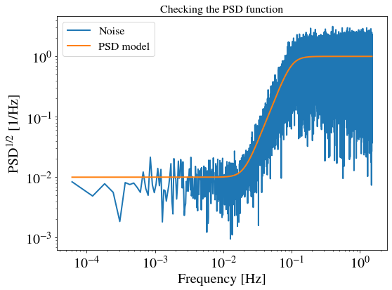
Check that the PSD function is consistent with the data

f = np.fft.rfftfreq(n_data) * fs
n_fft = np.fft.rfft(n)
psd = psd_function(f[f>0])
scalefac=np.sqrt(2 / (n_data*fs))
# Load plotting configuration
postprocess.plotconfig(lbsize=20, lgsize=16, autolayout=True, figsize=(8, 6),
                       ticklabelsize=20)
# Plot data against PSD
fig, ax = plt.subplots()
ax.set_title(r"Checking the PSD function")
ax.set_xlabel(r"Frequency [Hz]")
ax.set_ylabel(r"PSD${}^{1/2}$ [1/Hz]")
ax.loglog(f[f>0], np.abs(n_fft[f>0]) * scalefac, label="Noise")
ax.loglog(f[f>0], np.sqrt(psd), label="PSD model")
plt.legend()
plt.show()
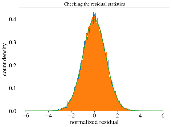
#Check the statistics on the residual
df=fs/n_data
nbins=int(np.sqrt(len(n_fft)))
plt.hist(n_fft.real[f>0]*scalefac/np.sqrt(psd/2),bins=nbins,density=True,label="real part")
plt.hist(n_fft.imag[f>0]*scalefac/np.sqrt(psd/2),bins=nbins,density=True,label='imag part')
x=np.linspace(-6,6,nbins)
plt.plot(x,norm.pdf(x))
plt.title(r"Checking the residual statistics")
plt.xlabel(r"normalized residual")
plt.ylabel(r"count density")
plt.show()

# Embed the PSD function in a class
class MyPSD(psdmodel.PSD):

    def __init__(self, n_data, fs):

        psdmodel.PSD.__init__(self, n_data, fs, fmin=None, fmax=None)

    def psd_fn(self, x):

        return psd_function(x)

# Instantiate the psd class
psd_cls = MyPSD(n_data, fs)

3. Instantiate the imputation class

Then, from the signal and noise models, we can instantiate the GaussianStationaryProcess class from the datamodel module:

# instantiate imputation class
imp_cls = datamodel.GaussianStationaryProcess(s, mask, psd_cls, method='nearest', na=50*fs, nb=50*fs)
# perform offline computations
imp_cls.compute_offline()
# If you want to update the deterministic signal (the mean of the Gaussian process)
imp_cls.update_mean(s)
# If you want to update the PSD model
imp_cls.update_psd(psd_cls)

Computation of autocovariance + PSD took 0.009068727493286133

4. Perform missing data imputation

We can then reconstruct the missing data with the impute method of the GaussianStationaryProcess class:

# Imputation of missing data by randomly drawing from their conditional distribution
t1 = time.time()
y_rec_draw = imp_cls.impute(y_masked, draw=True)
t2 = time.time()
print("Missing data imputation took " + str(t2-t1))

Missing data imputation took 3.5186729431152344

# Imputation of missing data by randomly drawing from their conditional distribution
t1 = time.time()
y_rec = imp_cls.impute(y_masked, draw=False)
t2 = time.time()
print("Missing data imputation took " + str(t2-t1))

Missing data imputation took 0.17664504051208496

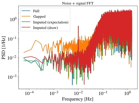
To see whether the imputation gives statisfactory statistics, we will compare the imputed data to the original one in Fourier domain. We start by Fourier-transforming the data:

# Fourier transform the results and the input data
y_fft = np.fft.rfft(y)
y_masked_fft = np.fft.rfft(y_masked)
y_rec_fft = np.fft.rfft(y_rec)
y_rec_draw_fft = np.fft.rfft(y_rec_draw)

# Plot results
fig, ax = plt.subplots()
ax.set_title(r"Noise + signal FFT")
ax.set_xlabel(r"Frequency [Hz]")
ax.set_ylabel(r"PSD [1/Hz]")
ax.loglog(f[f>0], np.abs(y_fft[f>0]) * scalefac, label="Full")
ax.loglog(f[f>0], np.abs(y_masked_fft[f>0]) * scalefac, label="Gapped")
ax.loglog(f[f>0], np.abs(y_rec_fft[f>0]) * scalefac, label="Imputed (expectation)")
ax.loglog(f[f>0], np.abs(y_rec_draw_fft[f>0]) * scalefac, label="Imputed (draw)")
plt.legend()
plt.show()

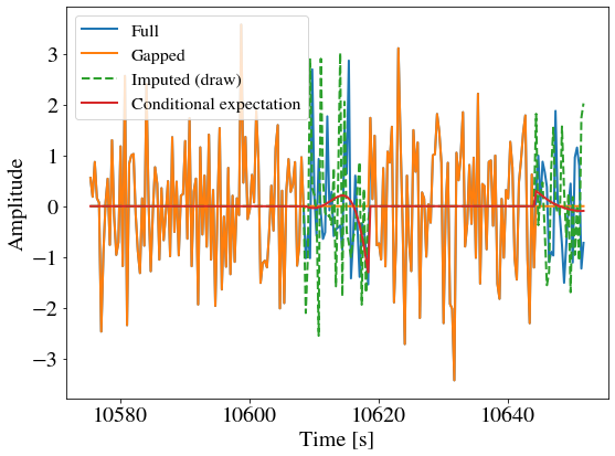
5. Comparing time series

k = 0
delta = 100
inds = np.arange(gapstarts[k]-delta, gapends[k]+delta)
ym = y * (1 - mask)
ym_rec_draw = y_rec_draw * (1 - mask)
var_rec_draw = np.var(ym_rec_draw[mask==0])
var_original = np.var(ym[mask==0])
print(var_rec_draw / var_original)

fig, ax = plt.subplots()
# ax.set_title(r"Noise + signal FFT")
ax.set_xlabel(r"Time [s]")
ax.set_ylabel(r"Amplitude")
ax.plot(t[inds], y[inds], label="Full")
ax.plot(t[inds], y_masked[inds], label="Gapped")
ax.plot(t[inds], ym_rec_draw[inds], label="Imputed (draw)", linestyle='dashed')
ax.plot(t[inds], y_rec[inds]* (1 - mask[inds]), label="Conditional expectation")
plt.legend()
plt.show()

1.0804432851355306

print(imp_cls.autocorr[0] / np.var(y) )

1.0000785973274076